This article presents a heuristic for mapping a real-valued random signal that follows an arbitrary distribution to a uniform distribution over \([0, 1]\). It’s based on maintaining \(n\) bins, each representing an equal slice of the distribution. The average values of the bins are used to define a piecewise linear mapping from the original distribution to the uniform distribution. The result is a function that normalizes any input signal onto \([0, 1]\). It also has the ability to adjust to changes in the distribution over time. A usage scenario is the normalization of ratings given by a particular judge into scores that can be compared from one judge to another, regardless of how harsh or generous the judges are.
Given \(n\) bins, the amortized cost of adding a sample to the model is \(O(\log n)\) and the cost of normalizing an input sample is \(O(\log n)\) as well.
We are concerned with the practical problem of normalizing ratings from an external source into consistent scores with a universal meaning. An external source might be a human assigning some sort of ratings or feedback, using a subjective scale. We would like to normalize those ratings such that their value has the same meaning,
The meaning of a score shall be its normalized rank or percentile, expressed as a value in the range \([0, 1]\). For example, if 23% of the input ratings are below 8.5 and the remaining 77% of ratings are above 8.5, then the normalized score for 8.5 is 0.23. Our goal is to build a function that takes input ratings and maps them to such normalized score. Input ratings are used in two ways:
This article focuses on the main idea behind the solution. The more tedious work such as the initialization phase or handling interpolation at the extremities of the distribution is published as part of the source code for our implementation.
Given a stream of input numbers, we have to build and maintain some data structure that models the input distribution, which we call the distribution tracker. We add new samples to the tracker in order to initialize or update the model. We also want to be able to obtain a normalized score by passing in a sample input without necessarily updating the tracker. This is summarized by the following OCaml interface:
type tracker
val add : tracker -> float -> unit
val normalize : tracker -> float -> float

(* Combine 'add' and 'normalize'. *)
val map : tracker -> float -> floatThe algorithm uses two main parameters:
A distribution tracker is made of \(n\) bins, each of which tracks an EMA. Updating the tracker is done by batches of \(n\) input samples. The algorithm is the following:
for i in 0 ... n - 1:
  acc[i] <- read_number()

sort(acc)

for i in 0 ... n - 1:
  update_ema(ema[i], acc[i])
As is, this algorithm requires \(n\) samples before the ema array could be initialized. Then it can be used to normalize any input sample.
In practice, we’d like to start normalizing samples on the fly, before seeing \(n\) samples. This is done during the initialization phase by sorting the array, whose length is \(i+1\) rather than \(n\), right after adding each sample. This shorter array can then be used in place of the normal array of length \(n\) for normalizing some input. Once this initialization phase is over, we sort the accumulator acc normally, just once every \(n\) samples.
The ema array provides \(n\) averages derived from input samples, which are guaranteed to be sorted in increasing order. Given an input sample to normalize, the two nearest bins are identified by some variant of binary search.
For accurate, tested algorithms, please refer to the OCaml implementation.
The uniformize program was used to apply the map function to each input sample.
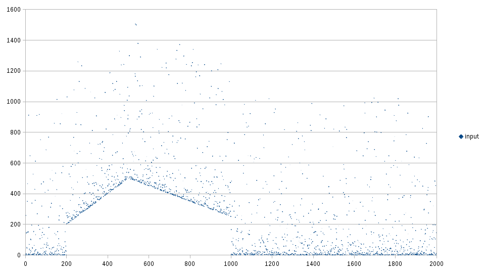
The following input signal was generated:
The samples are picked randomly using:
Using the parameters \(\alpha = 0.2\) and \(n = 20\), the results look as follows:
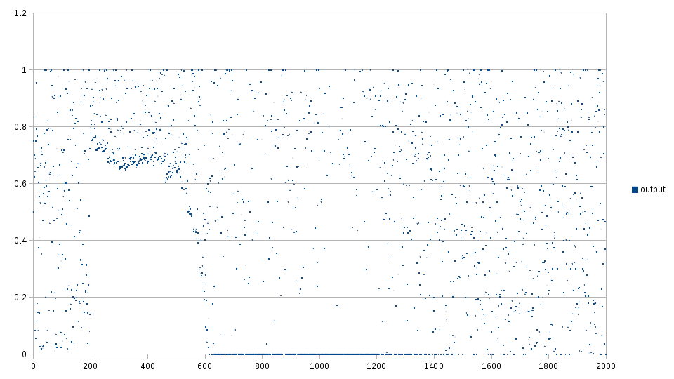
Normalization appears to give reasonable results fairly quickly from the beginning, as long as the distribution remains the same. However, it takes about 600 samples to recover from the changes in distribution once it stops changing (from sample 1000 to around 1600).
This implementation provides the missing details about the algorithms, unit tests, and a command-line program called uniformize: https://github.com/mjambon/uniformize