This document describes a moving average designed to reflect the current value of a signal most accurately. This is an improvement over exponential moving averages for some applications as it doesn’t require a trade-off between reactivity and smoothness.
Last revised: June 2018
This adaptive average was designed for signals that typically converge toward some stable value. Such signals initially increase, decrease, or oscillate at low frequencies. During these phases, it is more important for the application to track the latest values of the signal rather than the average over past values which are no longer relevant. However, once the signal stabilizes, we wish to remove noise as well as high frequency components.
Other practical goals shared with other moving averages are that the average can be computed at instant \(t\) without knowledge of the signal’s value beyond \(t\). Additionally, the algorithm must require very little memory, which makes window-based algorithms like a simple moving average not acceptable.
The adaptive average is defined as an exponential moving average of parameter \(\alpha\) where \(\alpha\) varies over time. The parameter \(\alpha\) at instant \(t\) is denoted \(\alpha_t\).
The exponential moving average \(m\) of a function \(f\) over nonnegative integers is defined as:
\[ m_{f, \alpha} = t \rightarrow \left\{ \begin{array}{ll} f_0 & t = 0\\ (1-\alpha_t) \cdot m_{f,\alpha}(t-1) + \alpha_t \cdot f_t & t > 0 \end{array} \right. \]
where
\[ \alpha_t = \max \left\{ \begin{array}{l} \frac{1}{t + 1} \\ \alpha \end{array} \right. \]
and \(\alpha\) is the user-defined parameter in the range \([0, 1]\) that controls how much weight is given to recent values.
That is, past some initial phase, \(\alpha_t\) is the constant \(\alpha\).
An exponential moving variance \(v\) is defined over positive integers as an exponential moving average of the squared difference between the signal \(f\) and the previous moving average of \(f\):
\[ \begin{eqnarray} v_{f, \alpha, \alpha^\prime} &=& m_{g, \alpha^\prime}\\ g &=& t \rightarrow (f_t - m_{f, \alpha}(t-1))^2 \end{eqnarray} \]
Note that \(v\) is not defined for \(t=0\). The moving standard deviation is defined as the square root of the moving variance.
The parameters \(\alpha\) and \(\alpha^\prime\) may be set to identical values but this is not a requirement.
The adaptive average \(M(f)\) of a signal \(f\) is defined like the exponential moving average, except that \(\alpha\) is no longer a constant. Several numerical parameters are involved but the default values that we use were found to work well and should be suitable for most applications. In what follows, \(m\) designates a classic exponential moving average.
The adaptive average \(M\) is updated at instant \(t\) as follows:
\[ M_t = \alpha_t \cdot f_t + (1-\alpha_t) \cdot M_{t-1} \]
\(\alpha\) now ranges between a minimum value \(\alpha_{\min}\) and a maximum \(\alpha_{\max}\) as follows:
\[\begin{eqnarray} \alpha_0 &=& \alpha_{\max} \\ \alpha_t &=& \max \left\{ \begin{array}{l} \alpha_{\min} + (\alpha_{\max} - \alpha_{\min}) \cdot I_t \\ \mathrm{maxshrink} \cdot \alpha_{t-1} \\ \end{array} \right. \\ \alpha_{\min} &=& 0.01 \\ \alpha_{\max} &=& 1 \\ \mathrm{maxshrink} &=& 0.9 \\ \end{eqnarray}\]
where \(I_t\) is the instability of the signal \(f\). It is defined as:
\[\begin{eqnarray} I_t &=& \left\{ \begin{array}{ll} \frac{1 + \mathrm{sign}(d_t) \cdot |d_t|^{\mathrm{lowpower}}}{2} & \mathrm{traveled}_t \neq 0\\ 1 & \mathrm{\mathrm{traveled}_t} = 0 \end{array} \right. \\ d_t &=& 2r_t - 1 \\ r_t &=& \frac{|\mathrm{elevation}_t|}{\mathrm{traveled}_t} \\ \mathrm{elevation} &=& m(\mathrm{slope}, \alpha_{gain}) \\ &=& \mathrm{gain} + \mathrm{loss} \\ \mathrm{traveled} &=& |\mathrm{gain}| + |\mathrm{loss}| \\ &=& \mathrm{gain} - \mathrm{loss} \\ \mathrm{gain} &=& m(\max(\mathrm{slope},0), \alpha_{\mathrm{gain}}) \\ \mathrm{loss} &=& m(\min(\mathrm{slope},0), \alpha_{\mathrm{gain}}) \\ \mathrm{slope}_t &=& \left\{ \begin{array}{ll} f_t - f_{t-1} & t \ge 0 \\ 0 & t = 0 \end{array} \right. \\ \mathrm{lowpower} &=& 0.5 \\ \alpha_{\mathrm{gain}} &=& 0.05 \\ \end{eqnarray}\]
Implementing this recipe requires tracking two exponential moving averages \(\mathrm{gain}\) and \(\mathrm{loss}\) of fixed parameter \(\alpha_{\mathrm{gain}}\). From these, the values of \(\alpha\) are determined at each time step.
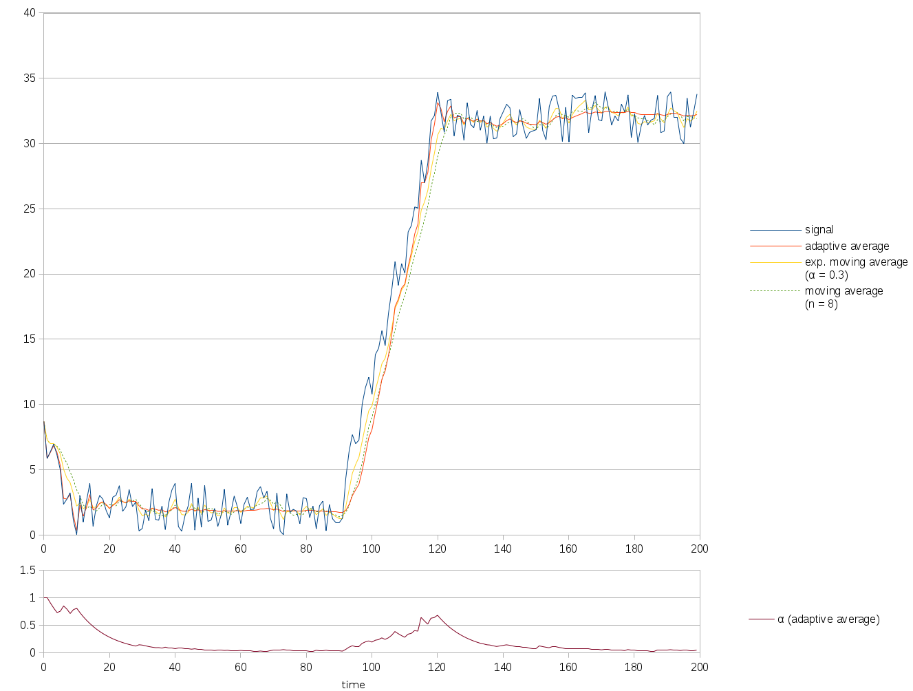
The graph below shows a signal that first decreases (steps 0-10) before stabilizing (steps 10-90). It then increases abruptly for some time (90-110) before stabilizing again. The values of \(\alpha\) as used in the adaptive average are plotted below the main graph.
Note how the adaptive average (solid red) follows the signal (solid blue) most closely in the following phases:
However, when the signal becomes stable, \(\alpha\) decreases despite the noise, unlike the classic moving average that uses a window of fixed length and unlike an exponential moving average of fixed parameter (steps 30-90, 130-200).
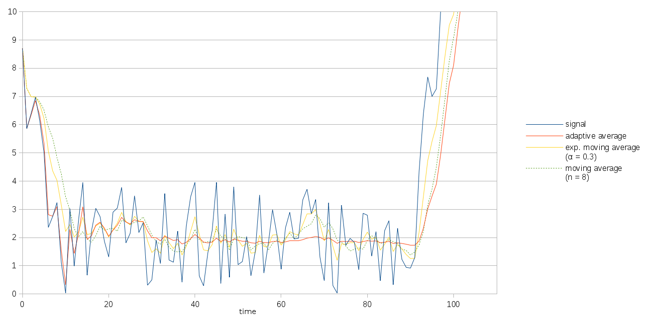
The following is an enlarged version of the first half of the graph:
At the time of writing, a sample implementation is available as part of https://github.com/mjambon/moving-percentile, as the modules Mv_adapt and Mv_adapt_avg.